Using Symbolic Mathematics with Optimization Toolbox Solvers
This example shows how to use the Symbolic Math Toolbox™ functions jacobian and matlabFunction to provide analytical derivatives to optimization solvers. Optimization Toolbox™ solvers are usually more accurate and efficient when you supply gradients and Hessians of the objective and constraint functions.
Problem-based optimization can calculate and use gradients automatically; see Automatic Differentiation in Optimization Toolbox. For a problem-based example using automatic differentiation, see Constrained Electrostatic Nonlinear Optimization Using Optimization Variables.
There are several considerations in using symbolic calculations with optimization functions:
Optimization objective and constraint functions should be defined in terms of a vector, say
x. However, symbolic variables are scalar or complex-valued, not vector-valued. This requires you to translate between vectors and scalars.Optimization gradients, and sometimes Hessians, are supposed to be calculated within the body of the objective or constraint functions. This means that a symbolic gradient or Hessian has to be placed in the appropriate place in the objective or constraint function file or function handle.
Calculating gradients and Hessians symbolically can be time-consuming. Therefore you should perform this calculation only once, and generate code, via
matlabFunction, to call during execution of the solver.Evaluating symbolic expressions with the
subsfunction is time-consuming. It is much more efficient to usematlabFunction.matlabFunctiongenerates code that depends on the orientation of input vectors. Sincefminconcalls the objective function with column vectors, you must be careful to callmatlabFunctionwith column vectors of symbolic variables.
First Example: Unconstrained Minimization with Hessian
The objective function to minimize is:
This function is positive, with a unique minimum value of zero attained at x1 = 4/3, x2 =(4/3)^3 - 4/3 = 1.0370...
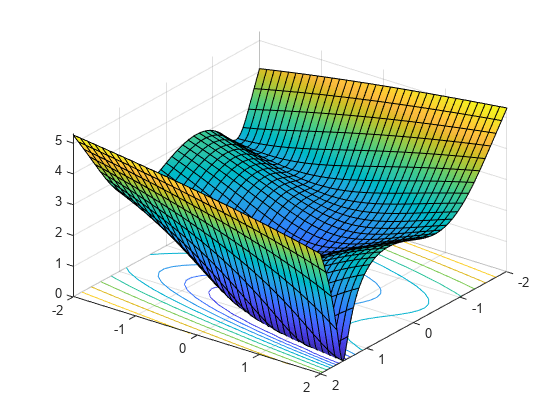
We write the independent variables as x1 and x2 because in this form they can be used as symbolic variables. As components of a vector x they would be written x(1) and x(2). The function has a twisty valley as depicted in the plot below.
syms x1 x2 real
x = [x1;x2]; % column vector of symbolic variables
f = log(1 + 3*(x2 - (x1^3 - x1))^2 + (x1 - 4/3)^2)
f =
fsurf(f,[-2 2],'ShowContours','on')
view(127,38)
Compute the gradient and Hessian of f:
gradf = jacobian(f,x).' % column gradfgradf =
hessf = jacobian(gradf,x)
hessf =
The fminunc solver expects to pass in a vector x, and, with the SpecifyObjectiveGradient option set to true and HessianFcn option set to 'objective', expects a list of three outputs: [f(x),gradf(x),hessf(x)].
matlabFunction generates exactly this list of three outputs from a list of three inputs. Furthermore, using the vars option, matlabFunction accepts vector inputs.
fh = matlabFunction(f,gradf,hessf,'vars',{x});Now solve the minimization problem starting at the point [-1,2]:
options = optimoptions('fminunc', ...
    'SpecifyObjectiveGradient', true, ...
    'HessianFcn', 'objective', ...
    'Algorithm','trust-region', ...
    'Display','final');
[xfinal,fval,exitflag,output] = fminunc(fh,[-1;2],options)
Local minimum possible.

fminunc stopped because the final change in function value relative to
its initial value is less than the value of the function tolerance.
xfinal = 2×1

    1.3333
    1.0370
fval = 7.6623e-12
exitflag = 3
output = struct with fields:
         iterations: 14
          funcCount: 15
           stepsize: 0.0027
       cgiterations: 11
      firstorderopt: 3.4391e-05
          algorithm: 'trust-region'
            message: 'Local minimum possible....'
    constrviolation: []
Compare this with the number of iterations using no gradient or Hessian information. This requires the 'quasi-newton' algorithm.
options = optimoptions('fminunc','Display','final','Algorithm','quasi-newton');
fh2 = matlabFunction(f,'vars',{x});
% fh2 = objective with no gradient or Hessian
[xfinal,fval,exitflag,output2] = fminunc(fh2,[-1;2],options)
Local minimum found.

Optimization completed because the size of the gradient is less than
the value of the optimality tolerance.
xfinal = 2×1

    1.3333
    1.0371
fval = 2.1985e-11
exitflag = 1
output2 = struct with fields:
       iterations: 18
        funcCount: 81
         stepsize: 2.1164e-04
     lssteplength: 1
    firstorderopt: 2.4587e-06
        algorithm: 'quasi-newton'
          message: 'Local minimum found....'
The number of iterations is lower when using gradients and Hessians, and there are dramatically fewer function evaluations:
sprintf(['There were %d iterations using gradient' ...
    ' and Hessian, but %d without them.'], ...
    output.iterations,output2.iterations)
ans =
'There were 14 iterations using gradient and Hessian, but 18 without them.'
sprintf(['There were %d function evaluations using gradient' ...
    ' and Hessian, but %d without them.'], ...
    output.funcCount,output2.funcCount)
ans =
'There were 15 function evaluations using gradient and Hessian, but 81 without them.'
Second Example: Constrained Minimization Using the fmincon Interior-Point Algorithm
We consider the same objective function and starting point, but now have two nonlinear constraints:
The constraints keep the optimization away from the global minimum point [1.333,1.037]. Visualize the two constraints:
[X,Y] = meshgrid(-2:.01:3);
Z = (5*sinh(Y./5) >= X.^4);
% Z=1 where the first constraint is satisfied, Z=0 otherwise
Z = Z+ 2*(5*tanh(X./5) >= Y.^2 - 1);
% Z=2 where the second is satisfied, Z=3 where both are
surf(X,Y,Z,'LineStyle','none');
fig = gcf;
fig.Color = 'w'; % white background
view(0,90)
hold on
plot3(.4396, .0373, 4,'o','MarkerEdgeColor','r','MarkerSize',8);
% best point
xlabel('x')
ylabel('y')
hold off
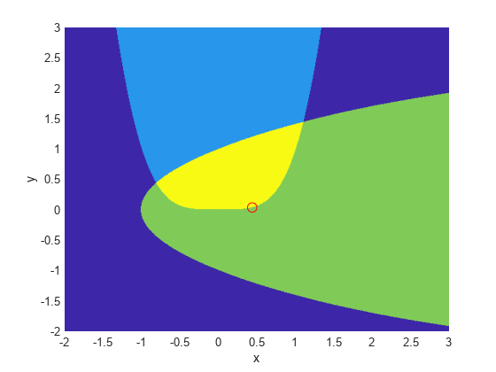
We plotted a small red circle around the optimal point.
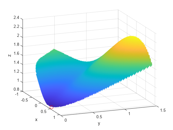
Here is a plot of the objective function over the feasible region, the region that satisfies both constraints, pictured above in dark red, along with a small red circle around the optimal point:
W = log(1 + 3*(Y - (X.^3 - X)).^2 + (X - 4/3).^2);
% W = the objective function
W(Z < 3) = nan; % plot only where the constraints are satisfied
surf(X,Y,W,'LineStyle','none');
view(68,20)
hold on
plot3(.4396, .0373, .8152,'o','MarkerEdgeColor','r', ...
    'MarkerSize',8); % best point
xlabel('x')
ylabel('y')
zlabel('z')
hold off
The nonlinear constraints must be written in the form c(x) <= 0. We compute all the symbolic constraints and their derivatives, and place them in a function handle using matlabFunction.
The gradients of the constraints should be column vectors; they must be placed in the objective function as a matrix, with each column of the matrix representing the gradient of one constraint function. This is the transpose of the form generated by jacobian, so we take the transpose below.
We place the nonlinear constraints into a function handle. fmincon expects the nonlinear constraints and gradients to be output in the order [c ceq gradc gradceq]. Since there are no nonlinear equality constraints, we output [] for ceq and gradceq.
c1 = x1^4 - 5*sinh(x2/5);
c2 = x2^2 - 5*tanh(x1/5) - 1;
c = [c1 c2];
gradc = jacobian(c,x).'; % transpose to put in correct form
constraint = matlabFunction(c,[],gradc,[],'vars',{x});
The interior-point algorithm requires its Hessian function to be written as a separate function, instead of being part of the objective function. This is because a nonlinearly constrained function needs to include those constraints in its Hessian. Its Hessian is the Hessian of the Lagrangian; see the User's Guide for more information.
The Hessian function takes two input arguments: the position vector x, and the Lagrange multiplier structure lambda. The parts of the lambda structure that you use for nonlinear constraints are lambda.ineqnonlin and lambda.eqnonlin. For the current constraint, there are no linear equalities, so we use the two multipliers lambda.ineqnonlin(1) and lambda.ineqnonlin(2).
We calculated the Hessian of the objective function in the first example. Now we calculate the Hessians of the two constraint functions, and make function handle versions with matlabFunction.
hessc1 = jacobian(gradc(:,1),x); % constraint = first c column
hessc2 = jacobian(gradc(:,2),x);

hessfh = matlabFunction(hessf,'vars',{x});
hessc1h = matlabFunction(hessc1,'vars',{x});
hessc2h = matlabFunction(hessc2,'vars',{x});
To make the final Hessian, we put the three Hessians together, adding the appropriate Lagrange multipliers to the constraint functions.
myhess = @(x,lambda)(hessfh(x) + ...
    lambda.ineqnonlin(1)*hessc1h(x) + ...
    lambda.ineqnonlin(2)*hessc2h(x));
Set the options to use the interior-point algorithm, the gradient, and the Hessian, have the objective function return both the objective and the gradient, and run the solver:
options = optimoptions('fmincon', ...
    'Algorithm','interior-point', ...
    'SpecifyObjectiveGradient',true, ...
    'SpecifyConstraintGradient',true, ...
    'HessianFcn',myhess, ...
    'Display','final');
% fh2 = objective without Hessian
fh2 = matlabFunction(f,gradf,'vars',{x});
[xfinal,fval,exitflag,output] = fmincon(fh2,[-1;2],...
    [],[],[],[],[],[],constraint,options)
Local minimum found that satisfies the constraints.

Optimization completed because the objective function is non-decreasing in
feasible directions, to within the value of the optimality tolerance,
and constraints are satisfied to within the value of the constraint tolerance.
xfinal = 2×1

    0.4396
    0.0373
fval = 0.8152
exitflag = 1
output = struct with fields:
         iterations: 10
          funcCount: 13
    constrviolation: 0
           stepsize: 1.9160e-06
          algorithm: 'interior-point'
      firstorderopt: 1.9217e-08
       cgiterations: 0
            message: 'Local minimum found that satisfies the constraints....'
       bestfeasible: [1x1 struct]
Again, the solver makes many fewer iterations and function evaluations with gradient and Hessian supplied than when they are not:
options = optimoptions('fmincon','Algorithm','interior-point',...
    'Display','final');
% fh3 = objective without gradient or Hessian
fh3 = matlabFunction(f,'vars',{x});
% constraint without gradient:
constraint = matlabFunction(c,[],'vars',{x});
[xfinal,fval,exitflag,output2] = fmincon(fh3,[-1;2],...
    [],[],[],[],[],[],constraint,options)
Local minimum found that satisfies the constraints.

Optimization completed because the objective function is non-decreasing in
feasible directions, to within the value of the optimality tolerance,
and constraints are satisfied to within the value of the constraint tolerance.
xfinal = 2×1

    0.4396
    0.0373
fval = 0.8152
exitflag = 1
output2 = struct with fields:
         iterations: 17
          funcCount: 54
    constrviolation: 0
           stepsize: 7.1892e-07
          algorithm: 'interior-point'
      firstorderopt: 3.8435e-07
       cgiterations: 0
            message: 'Local minimum found that satisfies the constraints....'
       bestfeasible: [1x1 struct]
sprintf(['There were %d iterations using gradient' ...
    ' and Hessian, but %d without them.'],...
    output.iterations,output2.iterations)
ans =
'There were 10 iterations using gradient and Hessian, but 17 without them.'
sprintf(['There were %d function evaluations using gradient' ...
    ' and Hessian, but %d without them.'], ...
    output.funcCount,output2.funcCount)
ans =
'There were 13 function evaluations using gradient and Hessian, but 54 without them.'
Cleaning Up Symbolic Variables
The symbolic variables used in this example were assumed to be real. To clear this assumption from the symbolic engine workspace, it is not sufficient to delete the variables. You must clear the assumptions of variables using the syntax
assume([x1,x2],'clear')All assumptions are cleared when the output of the following command is empty
assumptions([x1,x2])
ans =

Empty sym: 1-by-0
Related Topics
You can also select a web site from the following list:
Americas
- América Latina (Español)
- Canada (English)
- United States (English)
Europe
- Belgium (English)
- Denmark (English)
- Deutschland (Deutsch)
- España (Español)
- Finland (English)
- France (Français)
- Ireland (English)
- Italia (Italiano)
- Luxembourg (English)
- Netherlands (English)
- Norway (English)
- Österreich (Deutsch)
- Portugal (English)
- Sweden (English)
- Switzerland
- United Kingdom (English)